|
Material and methods
Chennai’s urban growth patterns have been assessed using temporal remote sensing data of Landsat satellite downloaded from public domains at Global Land Cover Facility (GLCF) (http://www.glcf.umd.edu/index.shtml) and United States Geological Survey (USGS) Earth Explorer (http://edcsns17.cr.usgs.gov/NewEarthExplorer/). Table 1 describes the data used, including remote sensing data and collateral data. The Survey of India (SOI) topographic maps of 1:50000 and 1:250000 scales were used to generate base layers such as the city boundary. Chennai’s administrative boundary is digitized from the city administration map obtained from the municipality. Ground control points to register and geo-correct remote sensing data were also collected using hand held pre-calibrated GPS (Global Positioning System) devices, Survey of India topographic maps and Google earth (http://earth.google.com, http://bhuvan.nrsc.gov.in). The method adopted to assess the urban growth patterns includes preprocessing, generation of land cover and land use and a gradient-wise zonal analysis of Chennai, is represented in Figure 2.
Preprocessing: The remote sensing data obtained was geo-referenced, geo-corrected, rectified and cropped pertaining to the study area. Remote sensing data from different sensors (with different spatial resolutions) was resampled to 30 m in order to maintain uniformity in spatial resolution. The study area includes the Chennai administrative area and 10 km buffer from the administrative boundary.
Data |
Year |
Purpose |
Landsat Series Thematic mapper (28.5m) |
1991, 2000 |
Land use, Land cover [LULC] analysis, landscape dynamics, urban growth patterns |
IRS P6 – LISS III MSS data (23.5m) |
2012 |
LULC analysis, landscape dynamics, urban growth patterns |
Survey of India (SOI) topographic maps of 1:50000 and 1:250000 scales |
|
To Generate boundary and Base layer maps. |
Field visit data –captured using GPS |
|
For geo-correcting and generating validation dataset |
Aster GDEM of1 arc-second(30 m) grid |
2010 |
Extraction of Drainage lines, Slope analysis. |
City developmental plans, location of various agents |
2005, 2015 |
Extraction of various agents of growth using Google earth and ancillary data |
Table 1: Data used in the Analysis
Land Cover Analysis: Land Cover analysis was performed to understand the changes in the vegetation cover during the study period in the study region. Normalized Difference Vegetation Index (NDVI) was found suitable and was used for measuring vegetation cover (Ramachandra et al., 2012a). NDVI values range from -1 to +1. Very low values of NDVI (-0.1 and below) correspond to soil or barren areas of rock, sand, or urban built up. Zero indicates the water cover. Moderate values (0.1 to 0.3) represent low-density vegetation, while high values (0.6 to 0.8) indicate thick canopy vegetation.
Land Use Analysis: Land use categories were classified using supervised technique with Gaussian Maximum Likelihood classifier (GMLC). The spatial data pertaining to different time frame were classified, using signatures from training sites for the land use types listed in table 2. The training polygons were compiled from collateral data of corresponding time period. Latest data were classified using signatures (training polygons) digitized with the help of Google earth. False color composite of remote sensing data (bands – green, red and NIR), was generated to visualise the heterogeneous patches in the landscape. 60% of the training data was used for classifying remote sensing data while the balance has been used for validation or accuracy assessment.
Land use Class |
Land uses included in the class |
Urban |
This category includes residential area, industrial area, all paved surfaces (road, etc.) and mixed pixels having major share of built up area. |
Water bodies |
Tanks, lakes, reservoirs. |
Vegetation |
Forest, nurseries. |
Others |
Rocks, cropland, quarry pits, open ground at building sites, un-metaled roads. |
Table 2: Land use classification categories adopted
Data is classified on the basis of training data through GMLC a superior method that uses probability and cost functions in its classification decisions (Duda et al., 2000; Ramachandra et al., 2012a). Mean and covariance matrices are computed using the maximum likelihood estimator. Land use was analysed using the temporal data retrieved from the open source program GRASS - Geographic Resource Analysis Support System (http://ces.iisc.ac.in/foss). Signatures were collected from field visit and Google earth. Classes of the resulting image were reclassified and recoded to form four land-use classes (Table 2).
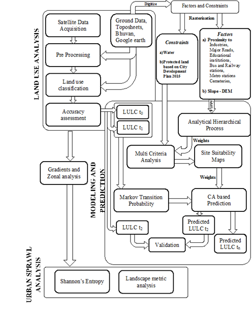
Figure 2: the procedure adopted for classifying the landscape and computation of metrics
Accuracy Assessment: Accuracy assessment has been done for the classified data to evaluate the performance of classifiers (Ramachandra et al., 2012a). This is done through using kappa coefficients (Congalton et al., 1983). Overall (producer and user) accuracies were computed through a confusion matrix. Assessing overall accuracy and computing Kappa coefficient are widely accepted methods to test the effectiveness of classifications (Lillesand and Kiefer, 2005; Congalton, 2009).
Zonal Analysis: The study area (city boundary with 10 km buffer region) is divided into 4 geographic zones based on direction– Northeast (NE), Southwest (SW), Northwest (NW) and Southeast (SE)– as a city or its growth is usually defined directionally. Zones were sub-divided using centroid as a reference (Central Business District). The growth of the urban areas in each zone was studied and understood separately, by computing urban density for different periods.
Gradient Analysis - (Division of zones into concentric circles): To visualise the process of urban growth at local levels and to understand the agents responsible for changes, each zone was divided into concentric circles that are 1 km apart and radiate from the city-center. The analysis of urban growth patterns at local levels help the city administrators and planners identify the causal factors of urbanization in response to the economic, social and political forces and visualizing the forms of urban growth with sprawl.
Urbanisation Analysis: To understand the growth of the urban area in specific zone and determine whether it is compact or divergent, the Shannon’s entropy (Sudhira et al., 2004; Ramachandra et al., 2012a) was computed for each zone. Shannon’s entropy (Hn), given in equation 1, explains the development process and its characteristics over a period of time and indicates whether the growth was concentrated or aggregated.
Computation of spatial metrics: Spatial metrics have been used to quantify spatial characteristics of the landscape. Selected spatial metrics were used to anlayse and understand the urban dynamics. FRAGSTATS (McGarigal and Marks in 1995) was used to compute metrics at three levels: patch level, class level and landscape level. Table 3. below gives the list of the metrics along with their description considered for the study.
Indicator |
Formula |
PLAND |
Pi = proportion of the landscape occupied by patch type i.
aij = area (m2) of patch ij, A = total landscape area (m2). |
Number of patches (Built-up) - NP |
, Range: NP≥ 1 |
Patch Density (PD) |
, Range: PD> 0 |
Largest patch Index (Built-up) (LPI) |
) , Range: 0< LPI≤ 100 |
Normalised landscape shape Index
(NLSI) |
Range: 0 to 1 |
Landscape shape Index (LSI) |
, Range: LSI≥1, without limit. |
Interspersion and Juxtaposition Index (IJI) |
Range: 0 < IJI ≤ 100
eik = total length (m) of edge in landscape between patch types I and k. m= number of patch type present in landscape. |
Clumpiness Index (Clumpy) |
Range: Clumpiness ranges from -1 to 1 |
Aggregation Index (AI) |
gii = number of like adjacencies (joins) between pixels of patch type (class) i based on the single-count method. max-gii = maximum number of like adjacencies (joins) between pixels of patch type (class) i based on the single-count method. |
Percentage of Like Adjacencies (PLADJ) |
gii = number of like adjacencies (joins) between pixels of patch type (class) i based on the double-count method.
gik = number of adjacencies (joins) between pixels of patch types (classes) i and k based on the double-count method. |
Patch Cohesion index |
|
Table 3: Landscape metrics used in the current analysis (McGarigal and Marks in 1995; Aguilera et al., 2011 Ramachandra et al., 2012a; 2015).
Visualisation of urban growth in Chennai by 2026: Agents of urbanisation and constraints (listed in table 4) with temporal land uses were taken as baselayers for modelling and visualisation. Data values were normalized through fuzzification wherein the new values ranged between 0 and 255, 255 indicating maximum probability of change in land use in contrast with 0 for no changes. Fuzzy outputs thus derived are then taken as inputs to AHP for different factors into a matrix form to assign weights. Each factor is compared with another in pair wise comparison followed by enumeration of consistency ratio which should be preferably less than 0.1 for the consistency matrix to be acceptable. Once weights are determined MCE was used to determine the site suitability considering two scenarios i). Restrictions based on City Development Plan (CDP); ii). As usual scenario without CDP. These suitability change maps were considered in the MC-CA model. Considering earlier land uses, transition potentials were computed using a Markovian process. Using and hexagonal CA Filter of 5 x 5 neighborhood with variable iteration at every step until a threshold is reached. Careful model validation through kappa statistics was conducted to assure accuracy in prediction and simulation. Built-up areas were predicted for 2012 were cross-compared with the actual built-up areas in 2012 using classified data. The kappa index of 0.9 shows a good agreement accuracy of the model. Future patterns of urban expansion were then simulated for the years 2026.
Agents |
Industries, proximities to roads, railway stations, metro stations, educational institutes, religious places etc. |
Constraints |
Drainage lines, slope, water bodies, costal regulated areas, catchment areas etc. |
Table 4: Agents and constraints considered for modelling |

